分类与 Logistic 回归
分类用来预测若干个离散值。目前我们仅关注二分分类 (binary classifcation) 即 y 只有两个值 0, 1。0,被称为负类 (negative class); 1 被称为正类 (positive class),或者有时被记为 “-“ 和 “+” , 对于一个训练样本, 给定 \(x^{(i)}\), \(y^{(i)}\) 也被称作为 label 标签。
Logistic 回归就是来预测二分类 0, 1 的一种回归学习算法。Logistic 回归与一般的线性回归主要不同是选择假设函数不一样。
Logistic 回归
改变我们的 hypothesis 形式, \(h_\theta(x) = g(\theta^Tx) = \frac{1}{1 + e^{-\theta^Tx}}\) , 即 \(g(z) = \frac{1}{1 + e^{-z}}\), \(g(z)\) 被称为 Logistic 函数或 Sigmoid 函数。 Sigmoid 函数有如下的性质:
\[\begin{aligned} g'(z) &= \frac{d}{dz}(\frac{1}{1 + e^{-z}}) \\&= \frac{1}{1 + e^{-z}} e^{-z} \\ &=\frac{1}{1 + e^{-z}} (1- \frac{1}{1 + e^{-z}}) \\ &= g(z)(1-g(z)) \end{aligned}\]给出样本的假设函数,怎样才能拟合出 \(\theta\) 那?尝试用概率知识对参数 \(\theta\) 进行极大似然估计。
在极大似然估计之前,让我们先写出样本的概率密度函数。固定 \(\theta\), 在给出 \(x^{(i)}\) 时, \(y^{(i)}\) 的离散概率分布为:
\[\begin{aligned} f(y^{(i)} = 0 \mid x^{(i)}; \theta) &= 1 - h_\theta(x) \\ f(y^{(i)} = 1 \mid x^{(i)}; \theta) &= h_\theta(x) \\ f(y^{(i)}\mid x^{(i)}; \theta) &= h_\theta(x)^ {y^{(i)}} (1 - h_\theta(x))^{1 - y^{(i)}} \end{aligned}\]写出样本的联合概率函数:
\[L(\theta) = L(Y\mid X; \theta) = \prod_{i=1}^{m} h_\theta(x)^ {y^{(i)}} (1 - h_\theta(x))^{1 - y^{(i)}}\]则有:
\[\ell(\theta) = \ln L(\theta) = \sum_{i=1}^{m} \ln h_\theta(x)^ {y^{(i)}} (1 - h_\theta(x))^{1 - y^{(i)}}\]求出 \(\ell(\theta)\) 的最大值,我们可以使用梯度上升的方法来求得,即先随机初始化下 \(\theta\) ,然后利用梯度上升更新规则 \(\theta_j := \theta_j + \alpha \frac{\partial}{\partial{\theta_j}}\ell({\theta})\) 来更新 \(\theta\)。
我们需要求出 \(\frac{\partial}{\partial{\theta_j}}\ell({\theta})\), 让我们假设仅有一个样本的情况,则:
\[\begin{aligned} \frac{\partial}{\partial{\theta_j}}\ell({\theta}) &= \frac{\partial}{\partial{\theta_j}} \ln [h_\theta(x)^y(1-h_\theta(x))^(1-y)] \\ &= \frac{\partial}{\partial{\theta_j}} [y \ln h_\theta(x) + (1-y) \ln (1 - h_\theta(x))] \\ &= \frac{\partial}{\partial{\theta_j}} [y \ln g(\theta ^ Tx) + (1-y) \ln (1 - g(\theta ^ Tx))] \\ &= [y \frac{1}{g(\theta ^ Tx)} - (1-y) \frac{1}{ (1 - g(\theta ^ Tx)}] \frac{\partial}{\partial{\theta_j}}g(\theta ^ Tx) \\ &= [y \frac{1}{g(\theta ^ Tx)} - (1-y) \frac{1}{ (1 - g(\theta ^ Tx)}] g(\theta ^ Tx)(1 - g(\theta ^ Tx) \frac{\partial}{\partial{\theta_j}} \theta^Tx \\ &= [y (1 - g(\theta ^ Tx) - (1-y)g(\theta ^ Tx)] x_j \\ &= (y-h_\theta(x))x_j \end{aligned}\]即有更新规则为:\(\theta_j := \theta_j + \alpha (y^{(i)}-h_\theta(x^{(i)}))x_j^{(i)}\) 。看起来和我们的 LMS 类似,但是却不是同一个算法。因为现在我们的假设 \(h_\theta(x^{(i)})\) 是一个非线性函数。但是更新规则的相似是巧合吗? 我们将在 GLM 广义线性模型中讨论这个话题。
算法实现
'''
下面是一个仅有两特征的 Logistic Demo
'''
import numpy as np
import matplotlib.pyplot as plt
# 加载数据
def loadDataset(file):
fr = open(file)
dataset = []
labels = []
for line in fr.readlines():
lineNums = line.strip().split()
labels.append(int(lineNums[-1]))
dataset.append([1.0, float(lineNums[0]), float(lineNums[1])])
return dataset, labels
# 计算 Sigmoid hypothesis value
def calcHypothesis(z):
return 1 / (1 + np.exp(-z))
# 批量梯度上升算法
def batchGradientAscend(dataset, labels, maxIter = 500, alpha = 0.001):
dataset = np.mat(dataset)
labels = np.mat(labels).transpose()
m, n = dataset.shape
weights = np.ones((n, 1))
for i in range(maxIter):
error = labels - calcHypothesis(dataset * weights)
weights = weights + alpha * dataset.T * error
return weights
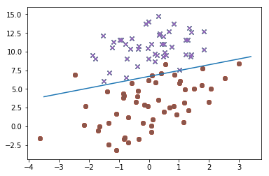
def plotLinear(dataset, labels, weights):
dataset = np.mat(dataset)
labels = np.array(labels)
negLabelsIndices = labels == 0
posLabelsIndices = labels == 1
negLabels = dataset[negLabelsIndices]
posLabels = dataset[posLabelsIndices]
plt.scatter(negLabels[:, 1], negLabels[:, 2], marker='x')
plt.scatter(posLabels[:, 1], posLabels[:, 2], marker='o')
x = np.arange(-3.5, 3.5, 0.1)
y = (-weights[0] - weights[1] * x) / weights[2]
plt.plot(x, np.squeeze(np.asarray(y)))
plt.show()
dataset, labels = loadDataset('./data/testSet.txt')
weights = batchGradientAscend(dataset, labels)
plotLinear(dataset, labels, weights)
运行结果
labels = [1, 0, 1, 0, 1]
amat = np.mat(labels)
arr = np.array(labels)
print(amat, amat.shape)
print(arr, arr.shape)
[[1 0 1 0 1]] (1, 5)
[1 0 1 0 1] (5,)